Part 2: Implementing Difference-in-Differences (DiD): A Practitioner’s Guide

Learn the practical mechanics of DiD - how to structure your data, validate assumptions, run fixed effects models, and communicate causal impact clearly.

and

Jun 24, 2025

👋 Hey! This is Manisha Arora from PrepVector. Welcome to the Tech Growth Series, a newsletter that aims to bridge the gap between academic knowledge and practical aspects of data science. My goal is to simplify complicated data concepts, share my perspectives on the latest trends, and share my learnings from building and leading data teams.

About the Authors:

Manisha Arora: Manisha is a Data Science Lead at Google Ads, where she leads the Measurement & Incrementality vertical across Search, YouTube, and Shopping. She has 12+ years of experience in enabling data-driven decision-making for product growth.

Banani Mohapatra: Banani is a seasoned data science product leader with over 12 years of experience across e-commerce, payments, and real estate domains. She currently leads a data science team for Walmart’s subscription product, driving growth while supporting fraud prevention and payment optimization. She is known for translating complex data into strategic solutions that accelerate business outcomes.

In the previous blog, we explored the intuition behind DiD, its core assumptions, real-world relevance, and evolution through key research milestones - laying a strong foundation for applying this method to product data science problems.

In this second part, we shift from “why” to “how.” We will walk through:

A step-by-step guide to implementing DiD, from data preparation to model estimation and interpretation
Risk factors and pitfalls where DiD might break down or yield misleading results

Whether you’re working with product experiments, feature launches, or staggered rollouts - this guide will help you structure a rigorous DiD analysis from start to finish.

Let’s dive in.

Step-by-step guide to implementing DiD

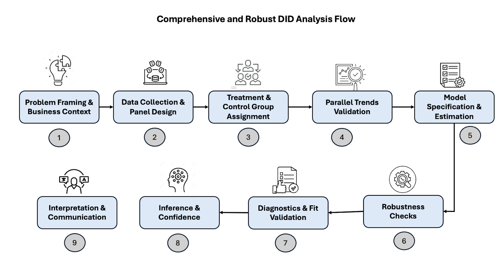
Step 1: Problem Framing & Business Context

Start by defining the business problem clearly:

What is the intervention?
When did it occur?
To whom was it applied?
Why does it matter to measure its impact?

This step guides every downstream decision including data design, control selection, and interpretation.

Things to keep in mind:

Clarify whether you're estimating ATT (Average Treatment on the Treated) or ATE (Average Treatment Effect).
Identify whether the treatment is a policy change, product feature, or marketing initiative.
Determine feasibility of finding control units and pre/post time windows.

Step 2: Data Collection & Panel Design

Build a panel dataset with repeated measurements over time for each observational unit (e.g., user, store, region).

What is panel data?

Panel data (also called longitudinal data) captures both cross-sectional and time-series dimensions. Each unit (e.g., a user or store) is tracked across multiple time points, allowing us to observe changes before and after treatment.

Example: Suppose you have user-level revenue data from January to June, along with a flag indicating if free shipping was available. You can structure the data like this:

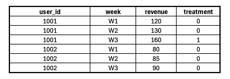
In this case:

user_id is the unit of observation.
week is the time dimension.
revenue is the outcome of interest.
treatment marks when the intervention was applied.

Panel Data Preparation Guidelines

To run a robust DiD analysis, your dataset should follow a panel (longitudinal) structure
Balanced panels, where each unit has data for every time period - are ideal for simplicity and consistent comparison. Unbalanced panels (with some unit-time gaps) are still usable. Just apply caution: use robust techniques like clustered standard errors, and check for any systematic missingness that could bias results.
Ensure enough pre-treatment periods to validate the parallel trends assumption.
Align your time granularity across the dataset (e.g., convert all data to weekly if needed).
Verify that all units are consistently tracked across time to prevent misclassification or dropout bias.

Step 3: Treatment & Control Group Assignment

At this stage, the goal is to identify which units are “treated” and which act as “controls.” This distinction is foundational for comparing changes over time and estimating causal effects. To build intuition, let’s walk through three common scenarios:

Scenario 1: Classic DiD (Clear Treated vs. Control)

In this traditional setup, the treatment and control groups are well-defined and fixed. For example, Store A receives a new feature rollout in March, while Store B does not. The groups remain stable throughout the study period, making the analysis straightforward with a single pre/post cutoff.

Scenario 2: All Users Exposed, Some Adopt

In some cases, all users are exposed to the intervention (e.g., free shipping), but only a subset actually engages with it. Here, “engagers” can be considered treated, and non-engagers as the control group. However, since engagement is self-selected and not randomized, this setup violates the core DiD assumption of exogenous treatment assignment.

This scenario is better handled using quasi-experimental designs like PSM or IPW. These methods create a synthetic control group by balancing pre-treatment characteristics, allowing for more credible causal inference despite the lack of randomization.

Scenario 3: Staggered Treatment

Sometimes treatment is rolled out at different times across units (e.g., Store A in March, Store B in April, Store C in May). In such cases, a single pre/post cutoff doesn’t apply. You’ll need multi-period DiD models or event study approaches to account for the varying treatment timing and to prevent biased estimates due to overlapping treatment windows.

Shameless plugs:

Product Data Science
Master Product Sense and AB Testing, and learn to use statistical methods to drive product growth. I focus on inculcating a problem-solving mindset, and application of data-driven strategies, including A/B Testing, ML, and Causal Inference, to drive product growth.

Check Out Product DS Course

AI/ML Projects for Data Professionals
Gain hands-on experience and build a portfolio of industry AI/ML projects. Scope ML Projects, get stakeholder buy-in, and execute the workflow from data exploration to model deployment. You will learn to use coding best practices to solve end-to-end AI and ML Projects to showcase to the employer or clients.

Step 4: Parallel Trends Validation

This assumption states that, in absence of treatment, the average outcomes for treated and control groups would have evolved similarly over time. This assumption enables us to attribute post-treatment differences in trends to the treatment itself, not pre-existing momentum or external factors.

If treated and control groups exhibit different trends before the intervention, any observed post-treatment effect could be due to pre-existing divergence rather than the treatment itself - leading to biased estimates.

How to Test

Visual Inspection

Plot the mean outcome over time for both treated and control groups. You should observe roughly parallel trajectories in the pre-treatment period. Divergence before treatment is a red flag.

Formal Statistical Test (Event Study / Leads & Lags Regression)

Introduce time-relative dummies (leads and lags) in the regression to test for pre-treatment differences:

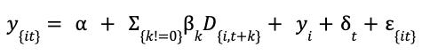
Where, D_{i,t+k} is an indicator for unit i being k periods away from treatment.

β_k (for k < 0) captures pre-treatment trends. These coefficients should not be statistically significant.
γ_i are unit fixed effects, δ_t are time fixed effects.
This model helps diagnose violations of the parallel trends assumption and reveals dynamic treatment effects over time.Step5: Model Specification & Estimation

Step 5: Model Specification & Estimation

Once we’ve validated the parallel trends assumption, we can formally estimate the treatment effect using a Difference-in-Differences (DiD) regression model.

The canonical DiD model is specified as:

y_it: Outcome variable for unit i at time t
treatment_i: Binary variable (1 if unit i is in the treatment group)
post_t: Binary variable (1 if time t is after treatment began)
treatment_i * post_t: Interaction term (1 only for treated units after treatment starts)
β_3: The DiD estimator – captures the Average Treatment Effect on the Treated (ATT)

Transformations:

TWFE: Two-Way Fixed Effects

In many applications, units (e.g., stores, users, zip codes) have inherent differences that don’t change over time - such as average sales levels or user behavior tendencies. Similarly, time periods may contain common shocks (e.g., holidays, macroeconomic changes) that affect all units. TWFE controls for both:

Unit-level fixed effects: Removes time-invariant differences between treated and control units.
Time fixed effects: Controls for any external factors affecting all units in a given time period.

This makes the DiD estimation cleaner by isolating the treatment effect from these confounding patterns.

Cluster standard errors

In panel data, outcomes from the same unit (e.g., the same store or user) tend to be correlated across time. If we ignore this and treat every observation as independent, our standard errors will be too small, and we may falsely declare results as statistically significant.

To fix this, we cluster standard errors by unit (or sometimes by region or group), which accounts for within-unit correlations. This ensures more reliable confidence intervals and p-values.

Clustered standard errors adjust for within-group correlation. They account for the fact that units within a group (cluster) are more similar to each other than to observations from other clusters.

Log-transform outcomes if skewed

When the outcome variable (like revenue or purchase value) is highly skewed, it can dominate the regression and reduce model performance. Applying a log transformation compresses extreme values, making trends more interpretable and the treatment effect easier to compare across units.

This is especially helpful when analyzing percentage changes or multiplicative effects, like “free shipping increased spend by 15%.”

You must handle zero or negative values carefully in this case, often by applying log(1 + y) or filtering them out.

Step 6: Robustness Checks

Even if your model shows a significant treatment effect, it’s critical to confirm that the result is genuine and stable.

1. Exclude Extreme Outliers

Sometimes, a few data points with unusually high or low values can disproportionately influence your estimates - especially in outcome variables like revenue or engagement.

Removing or winsorizing outliers ensures your results reflect the broader population, not rare events.

Example: If one store had an abnormally high sales day due to a local event unrelated to your feature rollout, including it could falsely exaggerate the treatment effect.

2. Placebo Tests (Fake Treatments)

To ensure your model is capturing a genuine causal effect rather than reacting to random fluctuations in the data, you can perform a placebo test using a fake treatment period that occurs before the actual intervention. This is similar to an A/A test in the RCT world, where no treatment is actually applied but the analysis is run as if there were one.

If you observe a significant treatment effect during this placebo window, it raises a red flag - suggesting that your model may be sensitive to background noise, mis-specified, or missing key confounders.

Example: Suppose your actual feature was launched in March. As a robustness check, pretend it was launched in February and rerun the DiD analysis. If you still observe a significant effect, it implies the model might be attributing changes to the treatment that are actually due to unrelated trends or seasonality.

3. Try Alternative Control Groups

Sometimes the control group you selected might differ in subtle but important ways from the treatment group. Trying different sets of control units - such as those in different geographies or customer segments - can help verify that your results aren’t overly dependent on one specific comparison.

Example: If you initially used stores in City B as a control for City A’s rollout, try using stores in City C to double-check consistency.

4. Vary the Pre/Post Time Window

Your results might depend heavily on how long you define the “before” and “after” periods. If the time window is too short, you might miss long-term effects; if it’s too long, other confounding changes might sneak in. By testing different window lengths, you can assess whether the treatment effect is robust across reasonable choices.

Example: Check the result using 2 weeks vs. 4 weeks pre/post windows to ensure the treatment signal holds steady.

5. Sensitivity Analysis on Covariates

If your model includes covariates (like user activity, demographic info, store size), test how the inclusion or exclusion of different combinations affects your results. Large swings in the treatment estimate may suggest that your model is sensitive to specification and may not be reliable.

Example: Run your DiD regression with and without session activity or annual purchase value to see if the treatment effect remains consistent.

Step 7: Diagnostics & Fit Validation

Once the model is estimated, it’s crucial to validate its underlying assumptions and check if it fits the data well.

Inspect residual plots to spot patterns that might indicate poor model fit or missing variables. Ideally, residuals should be randomly scattered.
Check for heteroskedasticity - when the variance of errors changes across observations - using tests like the Breusch-Pagan test. If present, standard errors may be biased.
Evaluate autocorrelation using tools like the Durbin-Watson statistic. If residuals are correlated over time, it can distort inference, especially in panel settings.
Confirm robustness by comparing results with alternative models - e.g., use Propensity Score Matching combined with DiD, or synthetic controls if applicable.

Step 8: Inference & Confidence

After estimation, quantify how confident you are in the results.

Report confidence intervals (typically 95%) to express the range within which the true effect likely falls.
Use clustered standard errors at the unit level (e.g., by store or region) to account for intra-group correlations, which are common in panel data.
Consider bootstrapping if your data violates model assumptions (e.g., non-normal residuals), as it provides a non-parametric way to estimate uncertainty.
Be cautious with p-values; use them as part of a broader inference strategy rather than the sole metric of significance.

Step 9: Interpretation & Communication

Translate technical results into insights that stakeholders can act on.

Express the estimated effect in business terms - such as additional revenue, conversion rate lift, or retention improvement.
Clearly explain the assumptions made (e.g., parallel trends) and the limitations of your analysis (e.g., data gaps, model sensitivity).
Include visualizations such as event study plots or time series comparisons to make trends and impacts easy to grasp.
Tailor your findings to different audiences by providing scenario-based insights (e.g., “the uplift in revenue was 1.5× higher in high-income zip codes”). This makes results more actionable for product, marketing, or strategy teams.

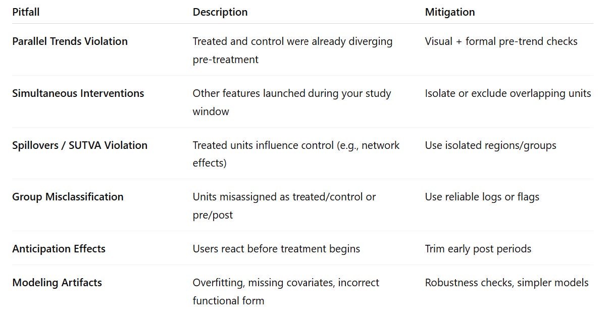
Risk Factors & Pitfalls in DiD

While Difference-in-Differences is a powerful tool for causal inference, it can yield misleading results if applied without care. Here are key scenarios where things may go wrong:

Violation of Parallel Trends:

If treated and control groups were already on different trajectories before the intervention, DiD estimates will be biased. Always inspect pre-treatment trends visually and statistically.

Simultaneous Interventions

When other features, campaigns, or external shocks occur during the study period (e.g., marketing push or policy change), they can confound your estimates. Be cautious of overlapping events and isolate the effect of interest.

Spillovers and Interference

If users in the control group are influenced by changes made to the treatment group (e.g., network effects or shared resources), the Stable Unit Treatment Value Assumption (SUTVA) is violated.

Incorrect Group or Time Assignment

Misclassifying units as treated/control or defining pre/post windows incorrectly can severely distort your results - especially in staggered rollouts. Use audit logs or flags to ensure accurate labels.

Anticipation Effects

If users change behavior before the intervention (e.g., expecting free shipping next week), early responses may bias your post-period effect. Trim or test early windows if necessary.

Modeling Artifacts

Overfitting, omitted variables, or inappropriate functional forms can produce spurious results. Run robustness checks like placebo tests, alternative control groups, or covariate sensitivity analysis to build confidence.

Coming Up Next: A Real-World Case Study

In the next blog, we’ll bring this methodology to life by applying it to a real-world business case study.

We’ll walk through simulations, visualizations, and step-by-step analysis, putting into practice everything we’ve covered so far, from assumptions to model design.

Upcoming Courses:

Product Data Science
Master Product Sense and AB Testing, and learn to use statistical methods to drive product growth. I focus on inculcating a problem-solving mindset, and application of data-driven strategies, including A/B Testing, ML, and Causal Inference, to drive product growth.