Propensity Score Matching: An Introduction for Data Scientists

An introduction to Propensity Score Matching, a tool for data scientists to reduce bias in observational studies and make reliable causal claims.

👋 Hey! This is Manisha Arora from PrepVector. Welcome to the Tech Growth Series, a newsletter that aims to bridge the gap between academic knowledge and practical aspects of data science. My goal is to simplify complicated data concepts, share my perspectives on the latest trends, and share my learnings from building and leading data teams

Imagine a scenario - You’re tasked with evaluating whether a new marketing campaign drove a measurable increase in customer conversion. It seems straightforward, but what if the data you’re working with isn't from a randomized experiment? You’re now facing the challenge of inferring causality from observational data.

About the Authors:

Manisha Arora: Manisha is a Data Science Lead at Google Ads, where she leads the Measurement & Incrementality vertical across Search, YouTube, and Shopping. She has 12+ years of experience in enabling data-driven decision-making for product growth.

Banani Mohapatra: Banani is a seasoned data science product leader with over 12 years of experience across e-commerce, payments, and real estate domains. She currently leads a data science team for Walmart’s subscription product, driving growth while supporting fraud prevention and payment optimization. She is known for translating complex data into strategic solutions that accelerate business outcomes.

Observational data, which comes from non-randomized settings, is full of biases that can distort our conclusions. This is why we need methods that can approximate the rigorousness of randomized controlled trials (RCTs), even when the data at hand isn’t derived from such an experiment. Propensity Score Matching (PSM) is one such method that enables data scientists to reduce selection bias and make more reliable causal inferences.

In our last post, we introduced the two foundational pillars of causal inference. One of them—Rubin’s Potential Outcomes Framework, also known as counterfactual reasoning—is built on a simple yet powerful question:

What would have happened to this individual if they had received a different treatment?

In randomized experiments, answering that is straightforward—we assign treatments randomly and compare outcomes. But in real-world business scenarios, randomization isn’t always practical, ethical, or even possible. That’s where causal inference methods come into play.

In today’s post, we’re zooming in on one of the most widely used approaches in this space: Propensity Score Matching (PSM). We’ll walk through a real-world example, break down how PSM works step-by-step, and show you how to implement it—yes, with both code and business context.

Let’s get into it!

The Fundamental Problem of Causal Inference

At the heart of causal inference lies a simple but profound problem:

We can never observe both potential outcomes for the same individual.

For a given unit, we either observe the outcome under treatment or under control — but never both. This missing data problem forces us to rely on assumptions and design strategies to approximate the missing counterfactuals.

For example, if a customer receives a new feature in your product, you can only observe how that individual behaves post-treatment, but you can’t see how they would have behaved had they not received the treatment (i.e., the counterfactual).

One naïve approach is to match individuals based on covariates — but as we'll see, simple covariate matching quickly falls apart in practice.

---

Shameless plugs:

1. Product Data Science

   Master Product Sense and AB Testing, and learn to use statistical methods to drive product growth. I focus on inculcating a problem-solving mindset, and application of data-driven strategies, including A/B Testing, ML, and Causal Inference, to drive product growth.

2. AI/ML Projects for Data Professionals

   Gain hands-on experience and build a portfolio of industry AI/ML projects. Scope ML Projects, get stakeholder buy-in, and execute the workflow from data exploration to model deployment. You will learn to use coding best practices to solve end-to-end AI and ML Projects to showcase to the employer or clients.

---

Matching Naively and Why It Fails

In theory, if we could find a control unit identical to every treated unit across all covariates, causal inference would be trivial. You might think that matching on similar covariates — such as age, location, income, etc. — could resolve this.

In practice, this is almost impossible for two reasons:

• Curse of Dimensionality: As the number of covariates increases, finding exact matches becomes exponentially harder.

• Bias-Variance Tradeoff: Relaxing matching criteria to find matches introduces bias; tightening them increases variance (fewer matches, noisier estimates).

Without controlling for confounding, the matched treatment and control groups may still differ significantly in terms of unobserved factors. Thus, naïve matching often results in biased estimates.

Enter Propensity Scores: The Key Idea

The solution to this problem is to reduce the dimensionality of the covariates by summarizing them into a single propensity score — the probability of receiving the treatment, given a set of observed covariates. Now, instead of matching on the full covariate set, we can match units on their propensity score. This is calculated using a model, typically logistic regression, where the treatment indicator (1 for treated, 0 for untreated) is regressed on the covariates.

Formally:

E(X)=P(Treatment=1∣X)

Under two assumptions:

1. Unconfoundedness: Treatment assignment is independent of potential outcomes conditional on covariates.

2. Overlap (Positivity): Every unit has a non-zero probability of being assigned to treatment or control.

→ Then, conditioning on the propensity score suffices to remove confounding bias.

In essence, the high-dimensional problem collapses into a one-dimensional balancing score.

Why does this work? By matching on the propensity score, you reduce the complexity of matching from potentially many dimensions to just one, making it computationally feasible and more effective in achieving balance between treated and control groups. The underlying assumption is that, once you account for the propensity score, the treatment assignment is random within strata of the score, meaning the observed covariates no longer confound the treatment effect.

Core Assumptions Behind Propensity Score Matching

For propensity score matching to provide a valid estimate of the treatment effect, several critical assumptions must hold:

• Unconfoundedness (Conditional Independence): This assumption states that, once we control for the propensity score, all confounders are accounted for. Essentially, it requires that there are no unobserved variables that simultaneously influence both the treatment assignment and the outcome.
  

• Overlap (Positivity): This assumption requires that for every combination of covariates, there’s a non-zero probability of receiving either treatment or control. If there are individuals with certain characteristics who are only ever treated (or never treated), then causal inference becomes impossible for those individuals because they have no counterfactual.

If these assumptions are violated, your propensity score estimates could be biased, and the causal claims you make from them might be invalid.

How Propensity Score Matching Works

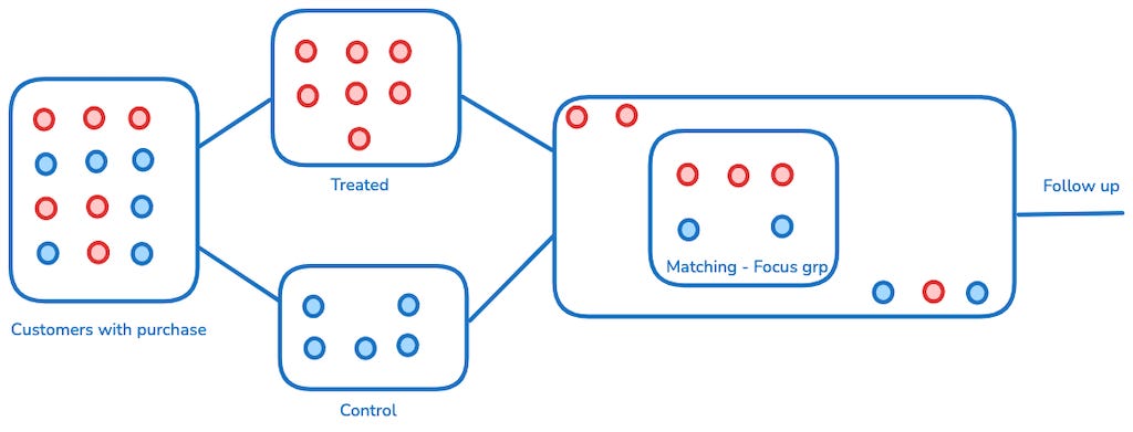
In practice, the steps for applying propensity score matching are straightforward, though the underlying complexity is in making sure the assumptions hold and that the methodology is applied properly. Here’s a simplified workflow:

1. Estimate Propensity Scores:
   You begin by estimating the propensity scores for all individuals in your dataset. This is typically done through a logistic regression or similar classification model, where the dependent variable is the treatment indicator and the independent variables are the covariates you want to control for.
   
   

2. Match Treated and Control Units:
   Once you have the propensity scores, you use these to match treated and control units. There are several matching algorithms you can use, such as nearest neighbor matching, caliper matching, or kernel matching, each with its trade-offs in terms of bias and variance.
   
   

3. Estimate Treatment Effect:
   After matching, the next step is to compare the outcomes of the treated and matched control units. This is where you can estimate the Average Treatment Effect on the Treated (ATT) — the causal effect of the treatment for those who actually received it.

4. Balance Check:

   It’s crucial to check if your matching procedure has effectively balanced the covariates between the treated and control groups. This can be done using statistical tests or visual methods like standardized mean differences or density plots. If balance is not achieved, you may need to refine your model or matching method.

What's Next

This introductory post only scratches the surface of what can be done with Propensity Score Matching. In future parts of this series, we’ll dive deeper into:

• Real-World Business Case: A detailed example applying PSM to measure the effect of a marketing campaign on customer conversion. We’ll walk through framing the business problem, designing the model, and analyzing the results.
  

• Practical Implementation: A hands-on guide using Python (with packages like sklearn and matchit) to perform the matching, estimate causal effects, and evaluate balance.
  

• Evaluation of Results: How to assess the robustness of your estimates, handle issues like lack of overlap, and perform sensitivity analysis to ensure your results hold up under scrutiny.

Stay tuned for the next edition!

---

Upcoming Courses:

1. Product Data Science

   Master Product Sense and AB Testing, and learn to use statistical methods to drive product growth. I focus on inculcating a problem-solving mindset, and application of data-driven strategies, including A/B Testing, ML, and Causal Inference, to drive product growth.

2. AI/ML Projects for Data Professionals

   Gain hands-on experience and build a portfolio of industry AI/ML projects. Scope ML Projects, get stakeholder buy-in, and execute the workflow from data exploration to model deployment. You will learn to use coding best practices to solve end-to-end AI/ML Projects to showcase to the employer or clients.

Not sure which course aligns with your goals? Send me a message on LinkedIn with your background and aspirations, and I'll help you find the best fit for your journey.