From Theory to Practice: Estimating the Causal Effect of Free Shipping Using IPW

We explore a real-world case study using Inverse Probability Weighting (IPW) to estimate the causal effect of free shipping on membership conversions — with step-by-step methodology, code, and results

and

May 29, 2025

👋 Hey! This is Manisha Arora from PrepVector. Welcome to the Tech Growth Series, a newsletter that aims to bridge the gap between academic knowledge and practical aspects of data science. My goal is to simplify complicated data concepts, share my perspectives on the latest trends, and share my learnings from building and leading data teams.

In our last edition, we introduced Inverse Probability Weighting (IPW) - a powerful technique to estimate causal effects from observational data by reweighting the population to mimic a randomized trial.

Today, we’re applying it to a real-world business scenario that’s common across many tech companies:

“Did offering free shipping cause more users to convert to paid memberships?”

A delivery service rolled out free shipping to all users as part of their membership program. But without a control group, traditional A/B testing was off the table. That’s where IPW comes in.

In this edition, we’ll walk through:

The business problem and why randomization wasn’t feasible
How to model treatment assignment and compute IPW weights
How to apply weights and assess balance
How to estimate the treatment effect and interpret results
Plus, the full codebase and diagnostics on GitHub

This is a hands-on, step-by-step walkthrough that bridges theory with execution — so you can start applying IPW to your own product and growth questions.

🧩 Choosing the Right Covariates

To answer our question — “Did offering free shipping cause more users to convert to paid memberships?” — we need to carefully select covariates that help us simulate a randomized experiment.

In inverse probability weighting (IPW), we model the probability that a user receives the treatment (free shipping) based on pre-treatment characteristics. These covariates must influence both:

The likelihood of receiving free shipping, and
The likelihood of converting to a paid membership

This helps us correct for confounding — ensuring that we're not mistaking correlation for causation.

Here are some candidate covariates to consider:

🔍 User Behavior & Engagement

Session activity: Total time spent, number of visits, or depth of interaction. More engaged users might be more likely to receive promotions and to convert.
Past trial behavior: Whether the user previously upgraded from a freemium plan.
Interactions with shipping promos: Views or clicks on shipping-related banners — a proxy for user interest.

🛒 Purchase & Spending History

Annual purchase value: High spenders may be prioritized for free shipping and may also have a higher likelihood of converting.
Order frequency or cart size: Indicates buying intent, which can influence both treatment and outcome.

📦 Membership Preferences

Membership plan (Monthly vs Annual): This could signal user intent and influence exposure to the free shipping offer.
Stage in trial (early/mid/late): Conversion likelihood often changes across a user’s trial journey.

🧑‍💻 User Profile

Geography or region: Free shipping may only be offered in select locations due to cost or logistics.
Device type: Mobile vs desktop could correlate with both treatment exposure and conversion behavior.
Tenure on platform: Long-standing users may behave differently from new sign-ups.

When selecting covariates, we follow the backdoor criterion from causal inference: include variables that influence both treatment and outcome, but avoid post-treatment variables, as they can introduce bias.

Covariate Summary Table:

To keep things simple for the rest of this blog, we have included 3 observed covariates :

Annual purchase value
Session activity
Membership plan type

In a previous post, we created matched pairs using PSM. Now, we’ll keep all users and reweight them based on how “typical” their treatment assignment was.

Shameless plugs:

Product Data Science
Master Product Sense and AB Testing, and learn to use statistical methods to drive product growth. I focus on inculcating a problem-solving mindset, and application of data-driven strategies, including A/B Testing, ML, and Causal Inference, to drive product growth.

Check Out Product DS Course

AI/ML Projects for Data Professionals
Gain hands-on experience and build a portfolio of industry AI/ML projects. Scope ML Projects, get stakeholder buy-in, and execute the workflow from data exploration to model deployment. You will learn to use coding best practices to solve end-to-end AI and ML Projects to showcase to the employer or clients.

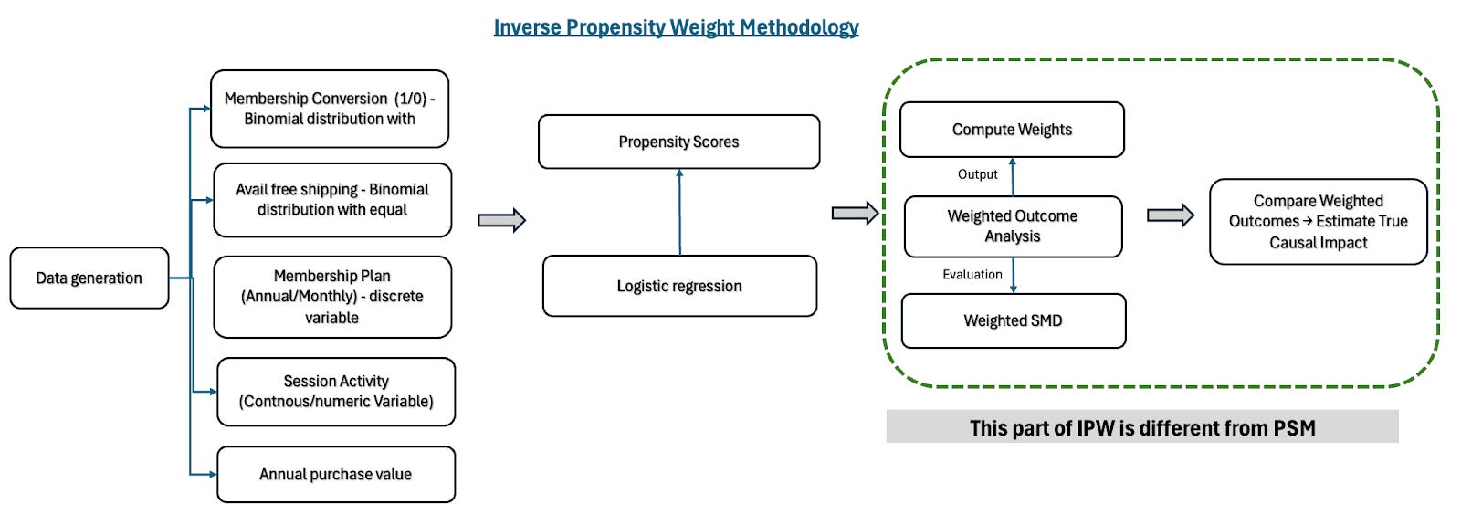
🧪 Methodology: How IPW Works (Step-by-Step)

This methodology outlines the Inverse Probability Weighting (IPW) approach used to estimate the causal impact of free shipping on membership conversion. The process involves data generation, propensity score estimation which is similar to PSM and the subsequent steps are different weight calculation, and applying weighted analysis to adjust for confounding, as illustrated in the diagram below.

As a refresher from the PSM blog, we simulated a dataset reflecting a real-world business scenario aimed at evaluating the impact of free shipping (treatment) on membership conversion (outcome). The data included key variables:

Outcome (Y): Membership conversion (1 = converted, 0 = not converted)
Treatment (T): Free shipping received (1 = yes, 0 = no)
Covariates (X):
- Membership Plan (X1): Annual or Monthly
- Session Activity (X2): User engagement level (continuous)
- Annual Purchase Value (X3): Total spending per year

Importantly, treatment assignment is confounded: users with higher spending or engagement are more likely to receive free shipping and to convert.

Step 1: Scoring the Odds – Estimating Propensity Scores (same as PSM)

Just like in PSM, we start by estimating each user’s propensity score—their likelihood of receiving free shipping based on observed characteristics like purchase value, session activity, and membership plan. We use logistic regression to predict the probability:

P(T=1∣X)=logistic(β0+β1X1+β2X2+β3X3)

This score tells us: “Given what we know about this user, how likely were they to get free shipping?” Every user ends up with a probability between 0 and 1.

Same starting point as PSM: We need these propensity scores to adjust for confounding—since more engaged or higher-spending users were both more likely to get free shipping and to convert.

Step 2: Weighting Instead of Matching – Creating Balance with Weights

Here’s where IPW diverges from PSM. Instead of trying to “find a match” for each treated user, we keep all users in the dataset and assign them a weight based on their propensity score.

Treated users (received free shipping) get a weight of:

wi=1pi

Control users (did not receive free shipping) get a weight of:

wi=11-pi

where pi is their estimated propensity score.

In the above approach, we upweight underrepresented users in each group—users who had a low chance of receiving treatment (but did) are given more weight, and users who had a high chance of not receiving treatment (but didn’t) are also given more weight. This process “rebalances” the groups statistically, making them comparable without excluding any observations.

Compared to PSM:

No units are dropped (PSM might discard unmatched users)
Everyone stays in the analysis, preserves statistical power
Balance is achieved by weighting rather than subsetting

Results:

The plot shows the distribution of propensity scores before and after applying IPW for treated and control groups. Initially (solid lines), treated and control groups had similar but not perfectly overlapping distributions, with treated users more concentrated around 0.32–0.36 and control users around 0.28–0.30. After weighting (dashed lines), the distributions aligned more closely, with better overlap and similar shapes between the groups.

Takeaway

IPW successfully balanced the treated and control groups, making their propensity score distributions more comparable. This balance supports the validity of causal effect estimates by reducing bias from observed confounders.

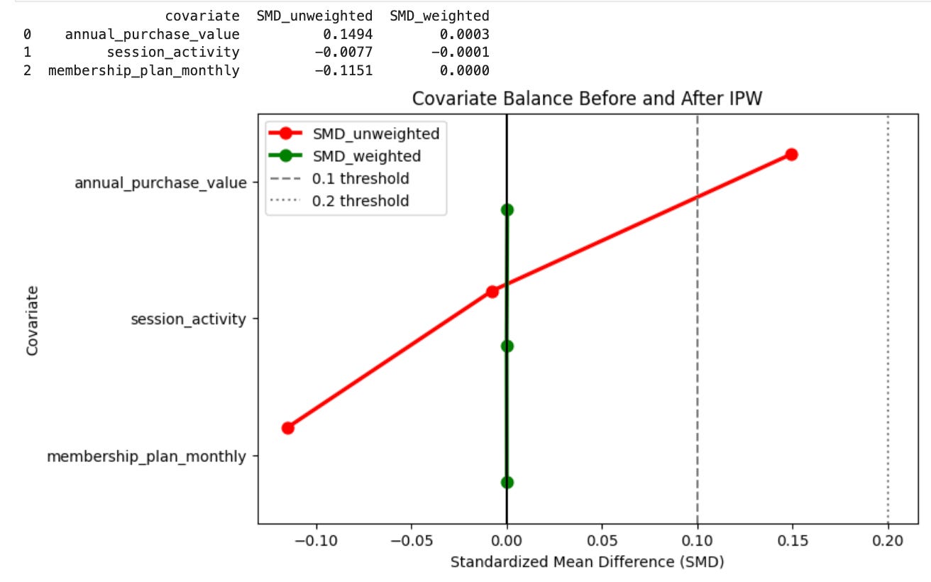
Step 3: Checking Balance with Weighted Covariates

Just like in PSM, we need to check: Did our adjustment successfully balance the covariates?

In PSM, we evaluate balance by comparing the covariates in the matched sample—after dropping unmatched units—whereas in IPW, we assess balance across all units by computing weighted means instead of simple averages. We calculate the standardized mean difference (SMD):

but here, both the means and the pooled standard deviation are derived from the weighted distributions. The interpretation remains the same:

SMD < 0.1 indicates excellent balance.
SMD < 0.2 indicates acceptable balance.

The goal is to make the weighted pseudo-population under IPW mimic a randomized experiment, just as PSM aims to create a balanced matched sample, ensuring treated and control groups are comparable across all observed variables.

Results

The plot shows that after applying IPW, all covariates achieved near-perfect balance with weighted SMDs close to zero and well below the 0.1 threshold. Before weighting, annual purchase value and membership plan showed mild imbalance, but IPW effectively reduced these differences.

Takeaway

IPW successfully balanced treated and control groups across all covariates.
The balance is exceptionally good—expected in a well-simulated dataset with strong overlap.
No immediate concerns, but in real data, such perfect balance might warrant checking for overfitting or limited covariate variability.

Step 4: Estimating Treatment Effect – Weighted Outcome Difference

Once balanced, we estimate the causal effect by calculating a weighted average outcome difference between treated and control users:

ATE = i T=1wiYii T=1wi-i T=0wiYii T=0wi

This weighted difference represents what the conversion rate would have been if the treated users had not received free shipping, adjusted for their underlying differences.

In PSM, we typically estimate ATT (Average Treatment Effect on the Treated) since matching focuses on treated units and asks, “What was the effect of treatment for those who actually received it?” In contrast, IPW can estimate either ATT or ATE, depending on how the weights are defined: weights restricted to treated units estimate ATT, while weights applied across both treated and control groups estimate ATE (Average Treatment Effect) for the entire population.

Interpretation:

Both PSM and IPW (ATT) estimate the treatment effect for users who received free shipping, but IPW yields a slightly higher effect (4.68% vs. 4.01%). This difference may stem from IPW retaining all treated samples through weighting rather than dropping unmatched pairs, resulting in greater statistical efficiency or subtle differences in balancing; alternatively, PSM’s exclusion of unmatched units could lower its estimate. Meanwhile, IPW (ATE) shows a slightly lower effect than IPW (ATT), suggesting free shipping was more impactful for those who actually received it compared to its effect across the entire population. This gap points to mild treatment effect heterogeneity—free shipping appears to benefit treated users a bit more than it would if offered universally.

Want to Dive Deeper? Explore the Code

We've shared the full implementation of this analysis on GitHub — from estimating propensity scores to computing the average treatment effect.

🔗 Access the Code on GitHub

You'll find:

Clean and modular Python code
Step-by-step comments for clarity
Visualizations to assess matching quality
Final estimation of the treatment effect

Feel free to fork, experiment, or adapt it to your use cases.

Wrapping It Up: What We Learned

Both PSM and IPW tell a consistent story: free shipping increases membership conversion by about ~4%. IPW delivers a slightly higher ATT estimate, likely due to retaining more data and variance among treated users. The difference between ATT and ATE under IPW reflects a marginally stronger effect for the treated group versus the broader population.

🔄 What’s Next?

But both these methods—PSM and IPW—share a key assumption: that all relevant confounders are observed and included in the model. In other words, they rely on “selection on observables.” But what happens when we worry about unobserved factors changing over time, or external shocks influencing both treatment and outcome?

That’s where Difference-in-Differences (DiD) enters the picture—a powerful causal method designed for panel data and pre-post comparisons. In our next post, we’ll explore how DiD can help estimate causal effects by leveraging changes over time, even in the presence of unobserved fixed confounders.

Stay tuned as we move from static comparisons to dynamic causal inference—and expand our causal toolkit with Difference-in-Differences.

Upcoming Courses:

Product Data Science
Master Product Sense and AB Testing, and learn to use statistical methods to drive product growth. I focus on inculcating a problem-solving mindset, and application of data-driven strategies, including A/B Testing, ML, and Causal Inference, to drive product growth.