

Part 3A: Measuring the Impact of Free Shipping: a Diff-in-Diff Case Study
Can free shipping truly drive growth? In this case study, we use Difference-in-Differences to measure its business impact.


👋 Hey! This is Manisha Arora from PrepVector. Welcome to the Tech Growth Series, a newsletter that aims to bridge the gap between academic knowledge and practical aspects of data science. My goal is to simplify complicated data concepts, share my perspectives on the latest trends, and share my learnings from building and leading data teams.
In Part 1 of this series, we introduced the Difference-in-Differences (DiD) method - unpacking its intuition, real-world relevance, and the core assumptions that make it work.
In Part 2, we provided a step-by-step guide to implementing DiD - from structuring panel data to model specification, validation, and inference.
Now, in Part 3, we bring it all together with a real-world-inspired case study.
Free shipping is a popular growth lever in e-commerce, often assumed to improve conversion and order value - but assumptions don’t equal impact. In this post, we’ll use DiD to estimate the causal effect of introducing free shipping for a subset of users over time.
You’ll learn how to:
Frame the business problem and define your treatment/control units
Build a panel dataset and validate the parallel trends assumption
Estimate treatment effects using fixed effects model
Let’s dive in.
Methodology:
In our last edition on IPW and PSM, the real-world case study we simulated addressed the question:
“Did offering free shipping cause more users to convert to paid memberships?”
We modeled this using static causal inference methods like PSM and IPW - both of which estimate treatment effects at a single point in time and are powerful when we can assume stable outcomes and limited temporal dynamics.
But business decisions rarely stop at conversion.
The broader question the business often asks is:
“Did offering free shipping lead to actual revenue growth from memberships, or did it merely shift fulfillment preference (e.g., from pickup to shipping)?”
This is where DiD steps in.
While PSM and IPW control for observed confounding in static settings, DiD is built to handle longitudinal, time-varying outcomes - like weekly revenue per user - and infer causal impact by comparing trends across treated and untreated groups over time.
Referring to the previously shared methodology flow,
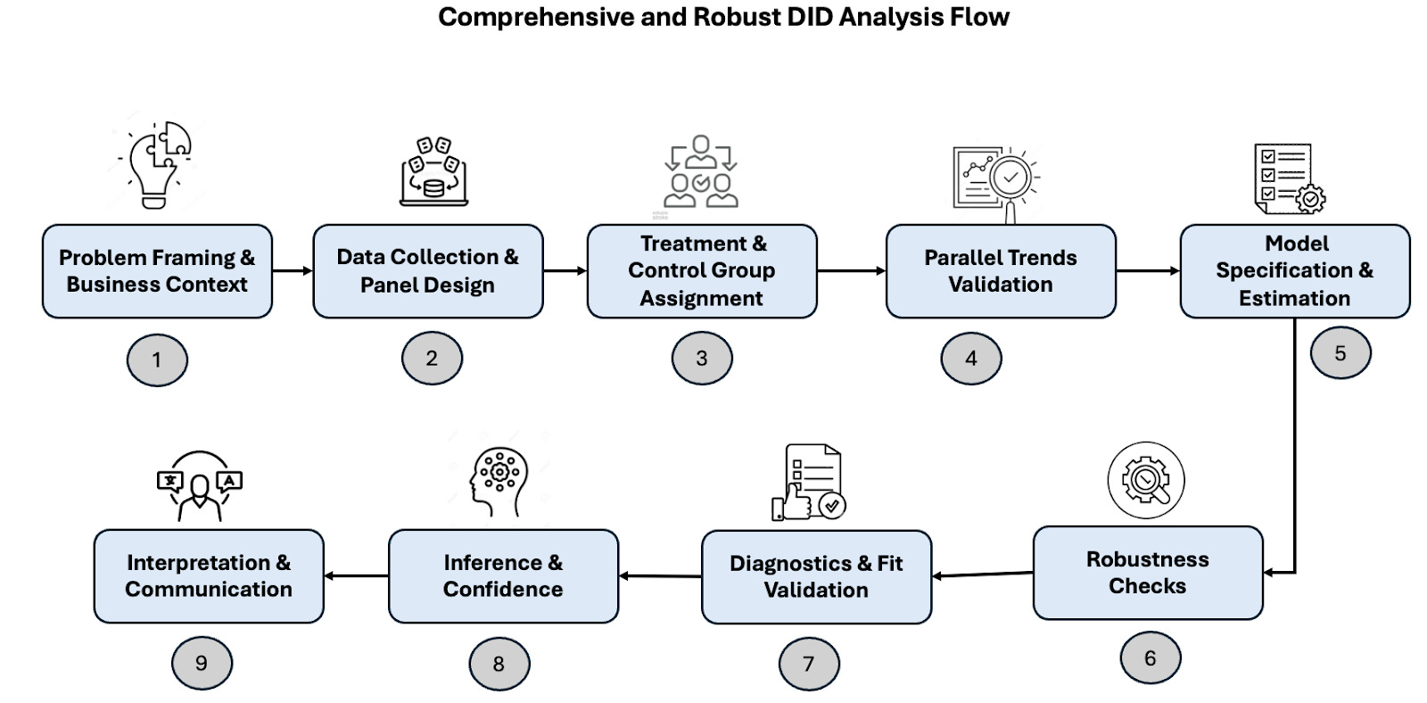
Step 1: Problem Framing & Business Context
The company introduced free shipping as a new benefit tied to its paid membership program. While early analysis showed an increase in membership signups, the business now wants to understand whether this feature led to a sustained lift in revenue - beyond short-term conversions.
In this case, we are estimating the Average Treatment Effect on the Treated (ATT) - specifically, the revenue uplift among users who actively used free shipping after subscribing.
This was a feature rollout made available to all users, but only a subset engaged with it. Since exposure was universal, a proper control group needs to be constructed - using non-engagers, matched via PSM based on pre-treatment revenue and user behavior.
We define weekly revenue per user for the 8 weeks before and after the launch. This temporal framing enables validation of the parallel trends assumption and supports the use of DiD to isolate the true effect of free shipping on revenue.
Step 2: Data Collection & Panel Design
To evaluate the revenue impact of free shipping using DiD, we first transformed our simulated user-level dataset into a balanced panel dataset. Each user (user_id) now appears in 16 weekly observations - 8 weeks before and 8 weeks after the intervention (week 9 onward). This structure enables us to track temporal changes in revenue for each user individually, which is fundamental to DiD.
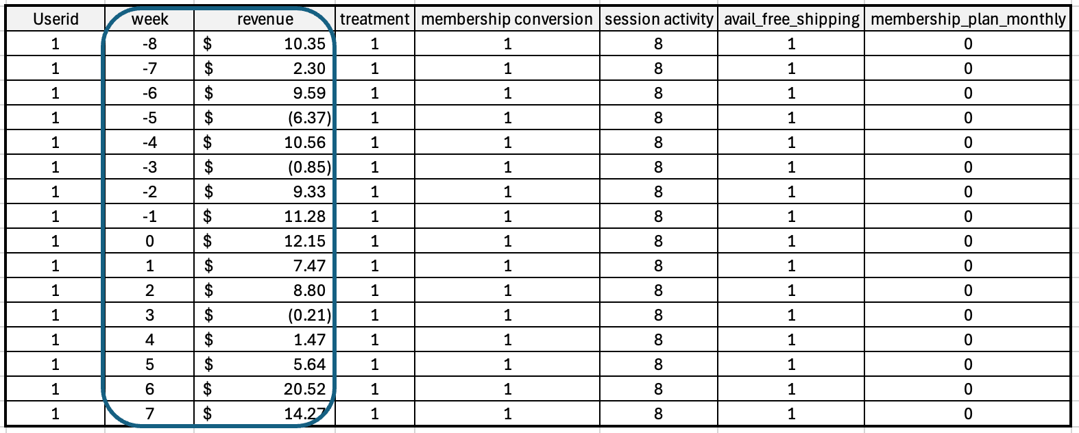
Figure: Structure of panel data for users classified as treated - i.e., those who used free shipping in the post-treatment period (Week 9 onwards).
Panel data (also known as longitudinal data) is a type of dataset that tracks multiple entities (like users, stores, or regions) over multiple time periods. It’s a data table where each row represents an entity at a point in time, allowing you to observe how that entity changes over time.
We followed these panel design guidelines:
Balanced panel: Every user has data across all 16 weeks - no missing unit-time observations.
Consistent granularity: Revenue is computed weekly for each user to ensure clean time comparisons.
Clear pre/post window: Weeks 1–8 are pre-treatment; weeks 9–16 are post-treatment.
Treatment variation: Users differ in exposure because only some adopted free shipping after it became available, enabling comparison of revenue trends between adopters and non-adopters.
No dropout or re-entry: All users are tracked uniformly, avoiding misclassification.
Shameless plugs:
Master Product Sense and AB Testing, and learn to use statistical methods to drive product growth. I focus on inculcating a problem-solving mindset, and application of data-driven strategies, including A/B Testing, ML, and Causal Inference, to drive product growth.
AI/ML Projects for Data Professionals
Gain hands-on experience and build a portfolio of industry AI/ML projects. Scope ML
Projects, get stakeholder buy-in, and execute the workflow from data exploration to model deployment. You will learn to use coding best practices to solve end-to-end AI and ML Projects to showcase to the employer or clients.
Step 3: Treatment & Control Group Assignment
In our simulated use case, free shipping was rolled out platform-wide, but only a subset of users actually used it. This aligns with Scenario 2: All Users Exposed, Some Adopt - a quasi-experimental design where treatment is defined not by exposure but by engagement.
Defining Treatment & Control in This Context:
Eligibility Window: All users became eligible for free shipping starting in week 9.
Treatment Group: Users who converted to paid membership and used free shipping during the post-rollout period. These users are considered treated (treatment = 1).
Control Group: Users who converted to paid membership but did not use free shipping. These users are considered controls (treatment = 0). Reasons may include not placing an order or choosing not to use the benefit.
Rationale: This setup ensures both groups have access to the same feature and membership status, isolating the effect of engagement with free shipping.
However, since treatment is not randomly assigned, we must ensure comparability between treated and control groups by adjusting for observed differences (like session activity or purchase value) using Propensity Score Matching (PSM) before applying DiD.
So, we implemented,
Simulated treatment assignment based on user attributes (annual_purchase_value, session_activity, membership_plan) to introduce realistic selection bias.
Created a binary treatment indicator in the panel dataset - active only in post-treatment weeks (week ≥ 9) for those marked as treated in the original data.
Ensured controls include users with similar characteristics but who did not adopt the feature.
Step 4: Parallel Trends Validation
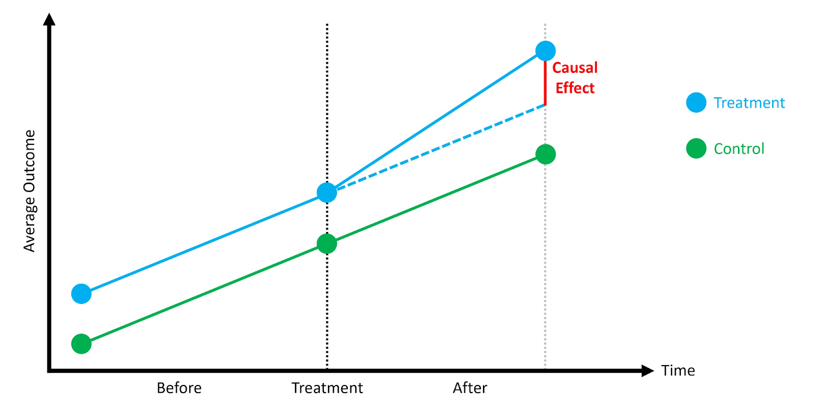
The parallel trends assumption is the backbone of the Difference-in-Differences method. It states that in the absence of treatment, the average outcomes for the treated and control groups would have followed similar trajectories over time.
Any difference we observe after the intervention can be attributed to the treatment — but only if both groups were on comparable paths before the treatment.
In our scenario, after identifying comparable treatment and control users using Propensity Score Matching, we constructed panel data tracking their revenue over time - 8 weeks before and after the free shipping rollout. The goal of this step was to ensure that the observed treatment effect isn’t just a continuation of pre-existing trends. If we had seen divergence before treatment, the results would be questionable, and DiD may not be valid.
But because we observed strong alignment before treatment and divergence only after, we gain confidence that the uplift is causal, not coincidental.
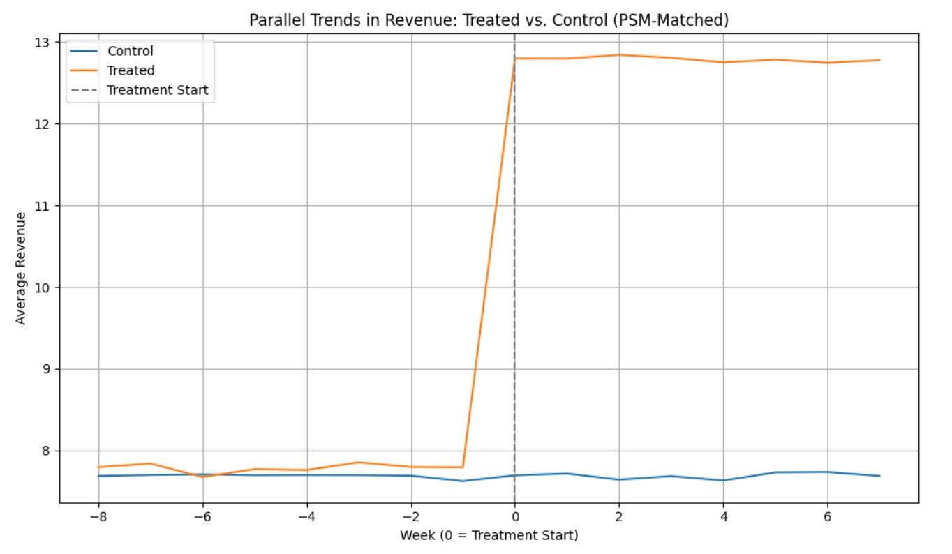
We then plotted average revenue per week for both groups to check if their trends were parallel before the treatment (week < 0).
How was it tested?
Visual Inspection
Pre-Treatment Period (Weeks -8 to -1):
The revenue trajectories of treated and control users were largely parallel - they moved together without major divergence.
This supports the Parallel Trends Assumption, the most critical assumption for valid Difference-in-Differences estimation.
Post-Treatment Period (Weeks 0 to 7):
The treated users began to show a noticeable revenue uplift relative to their matched control counterparts.
This difference can reasonably be attributed to the free shipping feature, assuming no other confounding events.
Formal Statistical Test (Event Study / Leads & Lags Regression)
To formally validate the parallel trends assumption in our difference-in-differences (DiD) setup, we used an event study regression that looks at user behavior over time - before and after the treatment.
2.1 Why not rely only on visual inspection?
While plotting average trends before and after treatment gives a quick sanity check, it’s subjective and may be distorted by:
Noise or outliers
Different scales across users
Aggregation artifacts
To overcome this, we used a fixed-effects panel regression with time-relative dummies, which provides a formal statistical test and gives week-by-week estimates of the treatment effect.
2.2 What is an event study in this context?
Think of it like tagging each user’s weekly behavior with how many weeks before or after treatment that observation occurred. For example, if a user first received free shipping in Week 0:
Week -2 becomes “2 weeks before treatment” (d_m2 = 1)
Week +3 becomes “3 weeks after treatment” (d_p3 = 1)
This timeline anchors user behavior to the moment of treatment, letting us compare across users treated at different times.
2.3 What we did (Step-by-step) and learnt?
For each user, we created dummy variables for each relative week (e.g., week = -6, -5, ..., +6). We excluded week = -1 as the baseline comparison period. We then ran a fixed-effects regression, which included:
User fixed effects: These account for each user’s overall behavior pattern. For example, some users consistently spend more than others. By using fixed effects, we compare each user to themselves over time, instead of comparing across users with different baseline behaviors.
Time fixed effects (optional): These are used to control for events or trends that affect everyone in a given week, such as seasonality or a platform-wide promotion. In our case, we removed time fixed effects to avoid overlap with the event-time dummy variables, which already capture week-by-week variation.
Clustered standard errors by user: Since we have repeated observations for each user, we cluster standard errors to account for correlation within a user’s behavior over time.
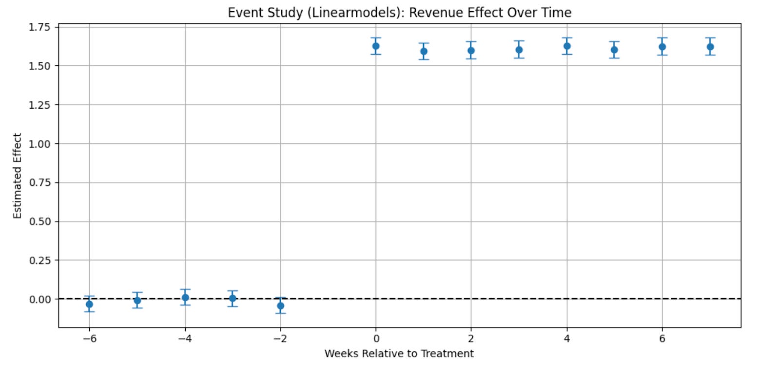
Figure: Output of the event study for revenue effect over time and users treated week
The chart shows how user revenue changed week by week, compared to just before they received free shipping.
The horizontal axis shows time, measured in weeks relative to when each user got free shipping. Week 0 is the moment treatment starts. Negative numbers are weeks before, and positive numbers are weeks after.
The vertical axis shows how much revenue changed compared to the baseline week (week -1).
Each dot represents the average estimated impact for that week.
The vertical lines around the dots show how confident we are in each estimate - shorter lines mean more certainty.
Interpretation:
Before treatment (weeks less than 0), the dots are close to zero, meaning revenue was stable and similar for treated and untreated users. That supports the idea that the groups were on parallel trends before the change. After treatment (week 0 and beyond), the dots jump up and stay high, which shows that free shipping had a clear and lasting positive effect on user revenue.
What’s Next?
In this blog, we covered steps 1-4 of DiD Implementation for the Free Shipping case study. In the next blog, we will go through steps 5 onwards.
Want to Dive Deeper? Explore the Code
We've shared the full implementation of this analysis on GitHub — from estimating propensity scores to computing the average treatment effect.
You'll find:
Clean and modular Python code
Step-by-step comments for clarity
Visualizations of the DiD model
Final estimation of the treatment effect
Feel free to fork, experiment, or adapt it to your use cases.
Upcoming Courses:
Master Product Sense and AB Testing, and learn to use statistical methods to drive product growth. I focus on inculcating a problem-solving mindset, and application of data-driven strategies, including A/B Testing, ML, and Causal Inference, to drive product growth.
AI/ML Projects for Data Professionals
Gain hands-on experience and build a portfolio of industry AI/ML projects. Scope ML Projects, get stakeholder buy-in, and execute the workflow from data exploration to model deployment. You will learn to use coding best practices to solve end-to-end AI/ML Projects to showcase to the employer or clients.
Not sure which course aligns with your goals? Send me a message on LinkedIn with your background and aspirations, and I'll help you find the best fit for your journey.
 | A guest post by
|